Plot the interaction in a single-equation time series model estimated via lm. It is imperative that you double-check you have referenced all x, y, z, and interaction terms through x.vrbl, y.vrbl, z.vrbl, and x.z.vrbl. You must also have their orders correctly entered. interact.adl.plot has no way of determining, from the variable list, which correspond with which

Plot the interaction in a single-equation time series model estimated via lm. It is imperative that you double-check you have referenced all x, y, z, and interaction terms through x.vrbl, y.vrbl, z.vrbl, and x.z.vrbl. You must also have their orders correctly entered. interact.adl.plot has no way of determining, from the variable list, which correspond with which

Usage

interact.adl.plot(
  model = NULL,
  x.vrbl = NULL,
  z.vrbl = NULL,
  x.z.vrbl = NULL,
  y.vrbl = NULL,
  effect.type = "impulse",
  plot.type = "lines",
  line.options = "z.lines",
  heatmap.options = "significant",
  line.colors = "okabe-ito",
  heatmap.colors = "Blue-Red",
  z.vals = NULL,
  s.vals = c(0, "LRM"),
  z.label.rounding = 3,
  z.vrbl.label = names(z.vrbl)[1],
  dM.level = 0.95,
  s.limit = 20,
  se.type = "const",
  return.data = FALSE,
  return.plot = TRUE,
  return.formulae = FALSE,
  ...
)

Arguments

model: the lm model containing the ADL estimates
x.vrbl: named vector of the “main” x variables and corresponding lag orders in the ADL model
z.vrbl: named vector of the “moderating” z variables and corresponding lag orders in the ADL model
x.z.vrbl: named vector with the interaction variables and corresponding lag orders in the ADL model. IMPORTANT: enter the lag order that pertains to the “main” x variable. For instance, x_l_1_z (contemporaneous x times lagged z) would be 0 and l_1_x_z (lagged x times contemporaneous z) would be 1
y.vrbl: named vector of the (lagged) y variables and corresponding lag orders in the ADL model
effect.type: whether impulse or cumulative effects should be calculated. impulse generates impulse effects, or short-run/instantaneous effects specific to each period. cumulative generates the accumulated, or long-run/cumulative effects up to each period (including the long-run multiplier). The default is impulse
plot.type: whether to feature marginal effects at discrete values of s/z as lines, or across a range of values through a heatmap. The default is lines
line.options: if drawing lines, whether the moderator should be values of z (z.lines) or values of s (s.lines). The default is z.lines
heatmap.options: if drawing a heatmap, whether all marginal effects should be shown or just statistically significant ones. (Note: this just sets the insignificant effects to the numeric value of 0. If the middle value of your scale gradient is white, these will effectively “disappear.” If another gradient is used, they will take on the color assigned to 0 values.) The default is significant
line.colors: what color lines would you like for line plots? This defaults to the color-safe Okabe-Ito (okabe-ito) colors. There is also a grayscale option through bw. Users can also include whatever colors they like. The number of colors must match the number of lines drawn. This is passed to scale_color_discrete
heatmap.colors: what color scale would you like for the heatmap? The default is Blue-Red. Alternate colors must be one of hcl.pals(). For grayscale plots, use Grays. This is passed to scale_fill_gradientn
z.vals: values for the moderating variable. If plot.type = lines, these are treated as discrete levels of z. If plot.type = heatmap, these are treated as a lower and upper level of a range of values of z. If none are provided, interact.adl.plot will pick
s.vals: values for the time since the shock. This is only used if line.options = s.lines, meaning s is treated as the moderator. The default is 0 (short-run) and the LRM
z.label.rounding: number of digits to round to for the z labels in the legend (if those values are automatically calculated)
z.vrbl.label: the name of the moderating z variable, used in plotting
dM.level: significance level of the (cumulative) marginal effects, calculated by the delta method. The default is 0.95
s.limit: an integer for the number of periods to determine the (cumulative) marginal effects (beginning at s = 0)
se.type: the type of standard error to extract from the model. The default is const, but any argument to vcovHC from the sandwich package is accepted
return.data: return the raw calculated (cumulative) marginal effects as a list element under estimates. The default is FALSE
return.plot: return the visualized (cumulative) marginal effects as a list element under plot. The default is TRUE
return.formulae: return the formulae for the (cumulative) marginal effects as a list element under formulae (for the (cumulative) marginal effects) and binomials (for the shock history). The default is FALSE
...: other arguments to be passed to the call to plot

Author

Soren Jordan, Garrett N. Vande Kamp, and Reshikesav Rajan

Examples

# Using Cavari's (2019) approval model
# Cavari's original model: APPROVE ~ APPROVE_ECONOMY + APPROVE_FOREIGN + MIP_MACROECONOMICS + 
#     MIP_FOREIGN + APPROVE_ECONOMY*MIP_MACROECONOMICS + APPROVE_FOREIGN*MIP_FOREIGN + 
#     APPROVE_L1 + PARTY_IN + PARTY_OUT + UNRATE + 
#     DIVIDEDGOV + ELECTION + HONEYMOON + as.factor(PRESIDENT)

approval$ECONAPP_ECONMIP <- approval$APPROVE_ECONOMY*approval$MIP_MACROECONOMICS
approval$FPAPP_ECONFP <- approval$APPROVE_FOREIGN*approval$MIP_FOREIGN

cavari.model <- lm(APPROVE ~ APPROVE_ECONOMY + APPROVE_FOREIGN + MIP_MACROECONOMICS + 
     MIP_FOREIGN + ECONAPP_ECONMIP + FPAPP_ECONFP + 
     APPROVE_L1 + PARTY_IN + PARTY_OUT + UNRATE + 
     DIVIDEDGOV + ELECTION + HONEYMOON + as.factor(PRESIDENT), data = approval)

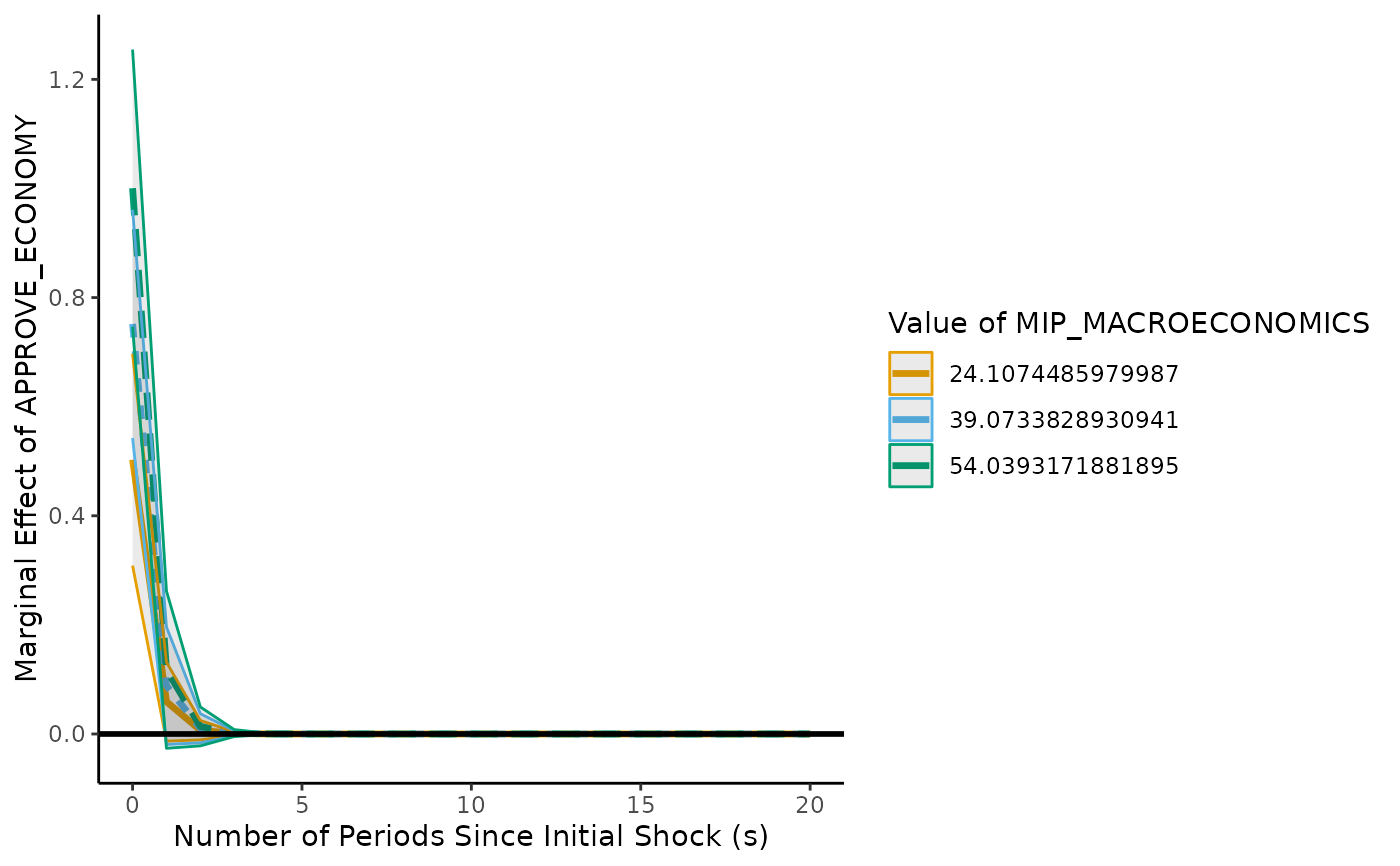
# Now: marginal effect of X at different levels of Z
interact.adl.plot(model = cavari.model, 
  x.vrbl = c("APPROVE_ECONOMY" = 0), y.vrbl = c("APPROVE_L1" = 1),
    z.vrbl = c("MIP_MACROECONOMICS" = 0), x.z.vrbl = c("ECONAPP_ECONMIP" = 0),
  effect.type = "impulse", plot.type = "lines", line.options = "z.lines")
#> Warning: Variable names containing . replaced with _


# Use well-behaved simulated data (included) for even more examples, 
#  using the Warner, Vande Kamp, and Jordan general model
model.toydata <- lm(y ~ l_1_y + x + l_1_x + z + l_1_z +
  x_z + z_l_1_x +
  x_l_1_z + l_1_x_l_1_z, data = toy.ts.interaction.data)

# Marginal effect of z (not run: computational time)
# Be sure to specify x.z.vrbl orders with respect to x term
if (FALSE) interact.adl.plot(model = model.toydata, x.vrbl = c("x" = 0, "l_1_x" = 1), 
        y.vrbl = c("l_1_y" = 1), z.vrbl = c("z" = 0, "l_1_z" = 1),
        x.z.vrbl = c("x_z" = 0, "z_l_1_x" = 1, 
          "x_l_1_z" = 0, "l_1_x_l_1_z" = 1),
        z.vals = -2:2,
        effect.type = "impulse", 
        plot.type = "lines", 
        line.options = "z.lines",
        s.limit = 20)
 # \dontrun{}

# Heatmap of marginal effects, since X and Z are actually continuous
#  (not run: computational time)
if (FALSE) interact.adl.plot(model = model.toydata, x.vrbl = c("x" = 0, "l_1_x" = 1), 
        y.vrbl = c("l_1_y" = 1), z.vrbl = c("z" = 0, "l_1_z" = 1),
        x.z.vrbl = c("x_z" = 0, "z_l_1_x" = 1, 
          "x_l_1_z" = 0, "l_1_x_l_1_z" = 1),
        z.vals = c(-2,2),
        effect.type = "impulse", 
        plot.type = "heatmap", 
        heatmap.options = "all",
        s.limit = 20)
 # \dontrun{}